Planning a MALDI Experiment using Analyte classes

Overview

MALDI-ToF can be used to gain insight into any chemical transformation that results in a change in mass. Additionally, multiple transformations can be simultaneously measured, given that the mass of each analyte is mass-resolved from the others.

The Analyte classes in MASSIVE can be used to programmatically define and visualize sets of analytes, with well-resolved mass distributions. This is conceptually similar to fluorophore choice when designing a flow cytometry panel.

This guide walks through an example using the Oligo class to visualize and refine a panel of oligonucleotides to measure activity in the context of enzymatic DNA synthesis.

---

Biochemistry context

In this example, we think through a MALDI experiment that tests for DNA polymerization by terminal deoxynucleotidyl transferase (TdT).

TdT naturally adds non-templated bases to the 3' end of a single-stranded DNA molecule, and is therefore of great interest in the field of enzymatic DNA synthesis. In order to limit the addition to a single nucleotide for use in sequence-specific synthesis schemes, it is necessary to add some sort of 3' blocker to the nucleotide being added, for example a phosphate group (3'phosphate-dGTP). However, it is known that the presence of a blocking group on the 3' end of a nucleotide interferes with the enzymatic activity of the enzyme. It is also known that TdT's enzymatic activity is dependent on both the sequence at the 3' end of the DNA that it is acting on, and the identity of the nuceotide being added.

With all of that in mind, we can imagine that it would be valuable to test for a couple of things simultaneously: - The activity of TdT on oligonucleotide substrates with varying 3' end sequences. - The activity of TdT with various 3' blocked nucleotides.

With MALDI, it is possible to measure every combination of these two properties simultaneously, assuming that each analyte is mass-resolved from the others. This principle can be extended to any molecular transformation that is mass-resolved.

Setup

from MASSIVE.analytes import Oligo
import matplotlib.pyplot as plt

Here are four nicely differentiated colours for our plots.

blue  = '#0072B2'
pink  = '#CC6677'
green = '#44AA99'
gold  = '#E69F00'

colours = [blue, pink, green, gold]

---

Step 1 — Define the base oligos

We will first define a set of four oligonucleotides that only differ by the 3' terminal base. If we test TdT polymerization on these oligos, we will get some information about its sequence preference.

base_oligos = [
    Oligo(name='base_3C', seq='GAAGACCACAACC'),  # blue
    Oligo(name='base_3T', seq='GAAGACCACAACT'),  # pink
    Oligo(name='base_3A', seq='GAAGACCACAACA'),  # green
    Oligo(name='base_3G', seq='GAAGACCACAACG'),  # gold
]

---

Step 2 — Check the mass distributions of the base oligos

Let's plot these oligos to see if they are mass-resolved. The Analyte.plot() method will automatically generate the isotopic distribution of each oligo, and if you know the resolution of the instrument you will use, the resolution parameter will allow you to estimate the actual signal distribution. If you don't know the resolution, you can leave this parameter blank or make a guess.

fig, ax = plt.subplots(figsize=(10, 2))

for i, o in enumerate(base_oligos):
    o.plot(ax=ax, label=o.name, colour=colours[i], mass_labels=False, resolution=5000)

ax.legend(bbox_to_anchor=(1.05, 1), loc='upper left')
ax.set_xlabel('m/z')
ax.set_ylabel('Relative intensity')

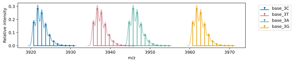
Notice: It's a bit tight, but these oligos are mass-resolved. If you were to run these together on MALDI, you would be able to quantify the relative abundance of each one. Great!

---

Step 3 — Check for overlap with polymerization products

In our assay, we want to polymerize each of the base oligos with all four dNTPs, and quantify the relative abundance of each product.

Below, we will plot the mass distributions of each oligo and its possible +1 products, with the colour corresponding to the base oligo.

We can add a 3'phosphate to the products, given that the experiment will use 3'phosphate-dNTPs.

fig, ax = plt.subplots(figsize=(10, 2))

polymerization_options = ['G', 'T', 'C', 'A']

for i, o in enumerate(base_oligos):

    o.plot(ax=ax, label=o.name, colour=colours[i], mass_labels=False)

    for N in polymerization_options:
        o_pol = Oligo(seq=o.seq + N, name=f"{o.name}{N}", mods=[o.mods, '3P'])
        o_pol.plot(ax=ax, label=o_pol.name, colour=colours[i], mass_labels=False)

ax.legend(bbox_to_anchor=(1.05, 1), loc='upper left')
ax.set_xlabel('m/z')
ax.set_ylabel('Relative intensity')

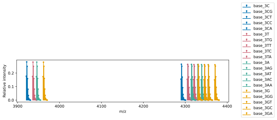
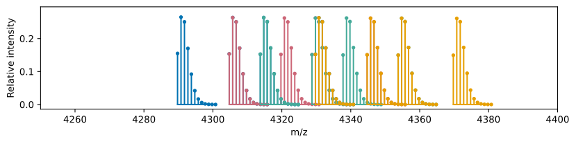
Yikes! The peaks from the polymerization reactions are overlapping. It would not be possible to work with this data.

---

Step 4 — Redesign to resolve conflicts

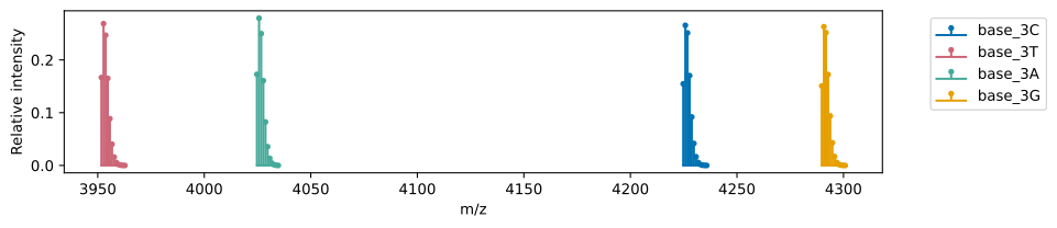
Fortunately, oligos can be readily synthesized with a variety of modifications, giving a lot of flexibility for where the masses will fall.

In the example below, we have made some minimal changes to the base oligos:

Oligo	Modification	Mass shift (Da)	Approx cost (USD)
3'C	5' dT	~320	<$1
3'T	1 phosphorothioate bond	~16	$4.50
3'A	5' phosphate	~80	$30
3'G	5' dG	~350	<$1

updated_oligos = [
    Oligo(name='base_3C', seq='TGAAGACCACAACC', mods=None),
    Oligo(name='base_3T', seq= 'GAAGACCACAACT', mods='PS'),
    Oligo(name='base_3A', seq= 'GAAGACCACAACA', mods='5P'),
    Oligo(name='base_3G', seq='GGAAGACCACAACG', mods=None),
]

---

Step 5 — Re-run the polymerization check

Now, let's visualize what the polymerization products look like with the new oligos.

fig, ax = plt.subplots(figsize=(10, 2))

for i, o in enumerate(updated_oligos):

    o.plot(ax=ax, label=o.name, colour=colours[i], mass_labels=False)

    for N in polymerization_options:
        o_pol = Oligo(seq=o.seq + N, name=f"{o.name}{N}", mods=[o.mods, '3P'])
        o_pol.plot(ax=ax, label=o_pol.name, colour=colours[i], mass_labels=False, resolution=5000)

ax.legend(bbox_to_anchor=(1.05, 1), loc='center left')
ax.set_xlabel('m/z')
ax.set_ylabel('Relative intensity')

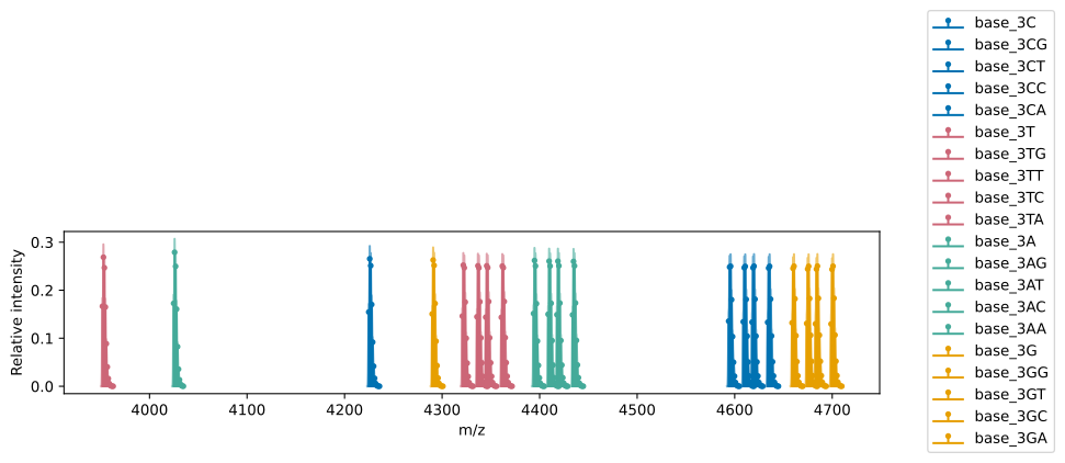
Note: Much better! Since we have spread out the base oligos, the polymerization products and each base oligo are now well-separated.

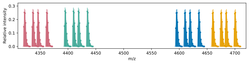
Here is the plot zoomed a bit closer to the polymerization products.

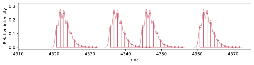
Zooming in further, we can see that each peak produces from polymerizing the base 3'T oligo is differentiated.

Quantitative simulations

Given that this experiment contains analytes with very similar masses, the question that arises is, what instrument resolution is required to comfortably differentiate these analytes?

We can answer this quantitatively using Analyte methods. MASSIVE can simulate signal distributions at a given resolution, and the Analyte.calc_signal_overlap() method allows two Analytes to be compared, returning the percentage overlap between the signals.

Here, we will compile all oligos into a single list, sort them by mass, then use Analyte.calc_signal_overlap() across a range of resolutions to determine the appropriate instrument requirements.

# collect all analytes into a single list
all_analytes = []
for o in updated_oligos:
    all_analytes.append(o)
    for N in polymerization_options:
        o_pol = Oligo(seq=o.seq + N, name=f"{o.name}{N}", mods=[o.mods, '3P'])
        all_analytes.append(o_pol)

# sort the list by mass
sorted_analytes = sorted(all_analytes, key=lambda o: o.monoisotopic_mass)

# define the parameters of the analysis
resolutions = range(1, 5000, 50)  # range of resolutions to consider
overlap_threshold = 0.01    # threshold for considering two oligos overlapping, they will be considered overlapping if their signal overlaps by at least 1%

def num_overlaps(resolution):   # function to count the number of oligos with overlapping signal at a given resolution
    num_overlaps = 0
    for i, o in enumerate(sorted_analytes):
        try:
            percent_overlap = o.calc_signal_overlap(sorted_analytes[i+1], resolution=resolution)
            if percent_overlap > overlap_threshold:
                num_overlaps += 1
        except IndexError:
            pass
    return num_overlaps

# calculate the number of overlaps at each resolution
overlaps = [num_overlaps(r) for r in resolutions]

# plot and format
fig, ax = plt.subplots(figsize=(7, 4))
ax.plot(resolutions, overlaps, marker='o', markersize=3)
ax.set_xlabel('Instrument resolution (R = m/Δm)')
ax.set_ylabel('Number of oligos with overlapping signal')
ax.set_title(f'Signal overlap vs. resolution, across entire set of oligos')

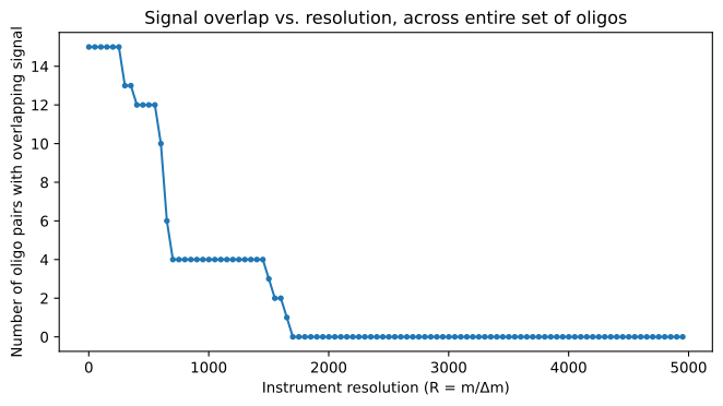
Result: We now know that these oligos can be unambiguously differentiated as long as the instrument has a resolution of ~2000 or greater.

With this information, let's go back and take a look at a cluster of analytes at 2000 resolution.

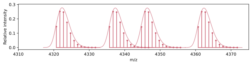
Looks about right! The tails of each distribution are very close to each other, but the peak of each distribution is clearly differentiated.

Summary

MASSIVE provides a flexible framework for defining and visualizing molecular analytes, along with quantitative analysis tools. In this example we have looked at how this can be applied to plan a highly-multiplexed activity assay for TdT, however, the principles of this guide can be applied to any situation where the user is interested in measuring chemical transformations via MALDI-ToF.